This is the first post in a series on how Slope's data-science team is using AI to improve the underwriting of small businesses. It starts with the layer of our stack where AI leverage is paying off most concretely today, the feature supply for our traditional underwriting ML model. A second post, coming next, will go one layer down to the bank-transaction labels that sit underneath all these features. For now, the topic is what an AI-driven research loop can produce when you point it at a well-defined credit-modeling problem.

Why I care about this problem

The underwriting model at Slope is a classical machine learning model. We chose it deliberately. When you decline a small business's application for financing, you have to be able to explain why. When a regulator or a partner bank asks how the model works, you need a solid answer. So we use a gradient-boosted tree model on a bounded set of features, every one of which a credit analyst could talk you through.

For a long time, the limiting factor on this model was the supply of features feeding it. Each good feature took about a week to produce. Research a hypothesis, implement it, backtest it, evaluate, iterate. Classical DS craft.

This post is about what happened when I asked: can the recent wave of AI tooling help me improve the feature supply to this model, without giving up the things that make it defensible?

As a DS working in 2026, I get to stand on a lot of shoulders, most notably Andrej Karpathy's auto-research loop, the agentic coding tools my teammates at Slope have been building, and a decade of credit risk thinking inside this company. This is a small report on what happens when you point them at a concrete business underwriting problem.

The ceiling of hand-crafted feature engineering

The old process was textbook. A DS reviews delinquency cases, notices a pattern, forms a hypothesis (e.g., "businesses that pay their lenders on time even when revenue is weak are healthier than their balance sheets suggest"), then engineers a feature that captures it, backtests it against historical data, and ships it if it clears the bar. Good craft. Every feature carried a story.

But there are two structural ceilings to working this way.

Human bandwidth. One principled feature, per analyst, per week, if you're being ambitious. That compounds slowly. In the time it takes to build out one angle, like the interaction between margin stability and debt service, half a dozen others sit unexplored on the whiteboard.

Hypothesis bias. You can only test ideas you've already thought of. And the delinquency cases you form hypotheses from are sparse, idiosyncratic, and anchored to the failure modes your team happens to encounter. Over time the feature portfolio becomes heavy on the signals you already suspected mattered, and thin on the ones you didn't know to look for.

We had started to feel this ceiling. Marginal features were getting harder to find. The model performed consistently well in the customer segments we'd personally investigated and less well in the ones we hadn't. We knew our approach was fundamentally correct, so the question became, "is there a way to run this same principled process at a much higher cadence?"

What Karpathy's auto-research showed us

Karpathy's autoresearch project demonstrated something simple but important. An AI agent can drive a research loop end-to-end if you give it three things: a clean quantitative metric, a reproducible sandbox, and a memory of what it's tried. The agent proposes, runs, evaluates, reads its own result, updates its notes, and iterates. The human supervises the direction rather than executing each step.

Adapting this to credit feature research took a specific framing: the agent is not inventing features from nothing. It is reasoning through the same first principles a human credit analyst would (revenue quality, margin, debt burden, expense structure, distress signals) at a cadence a human can't match and without the fatigue that narrows a tired analyst's hypothesis space.

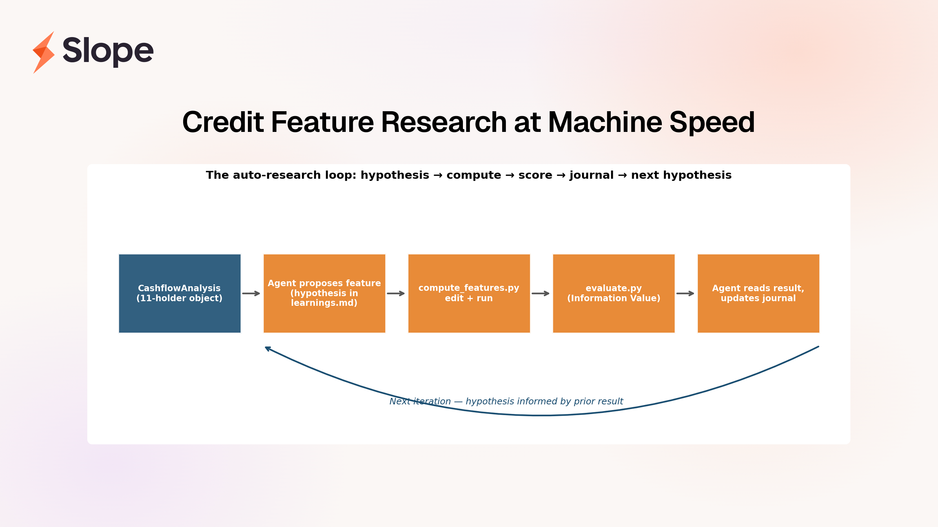
The loop we ended up with looks like this:

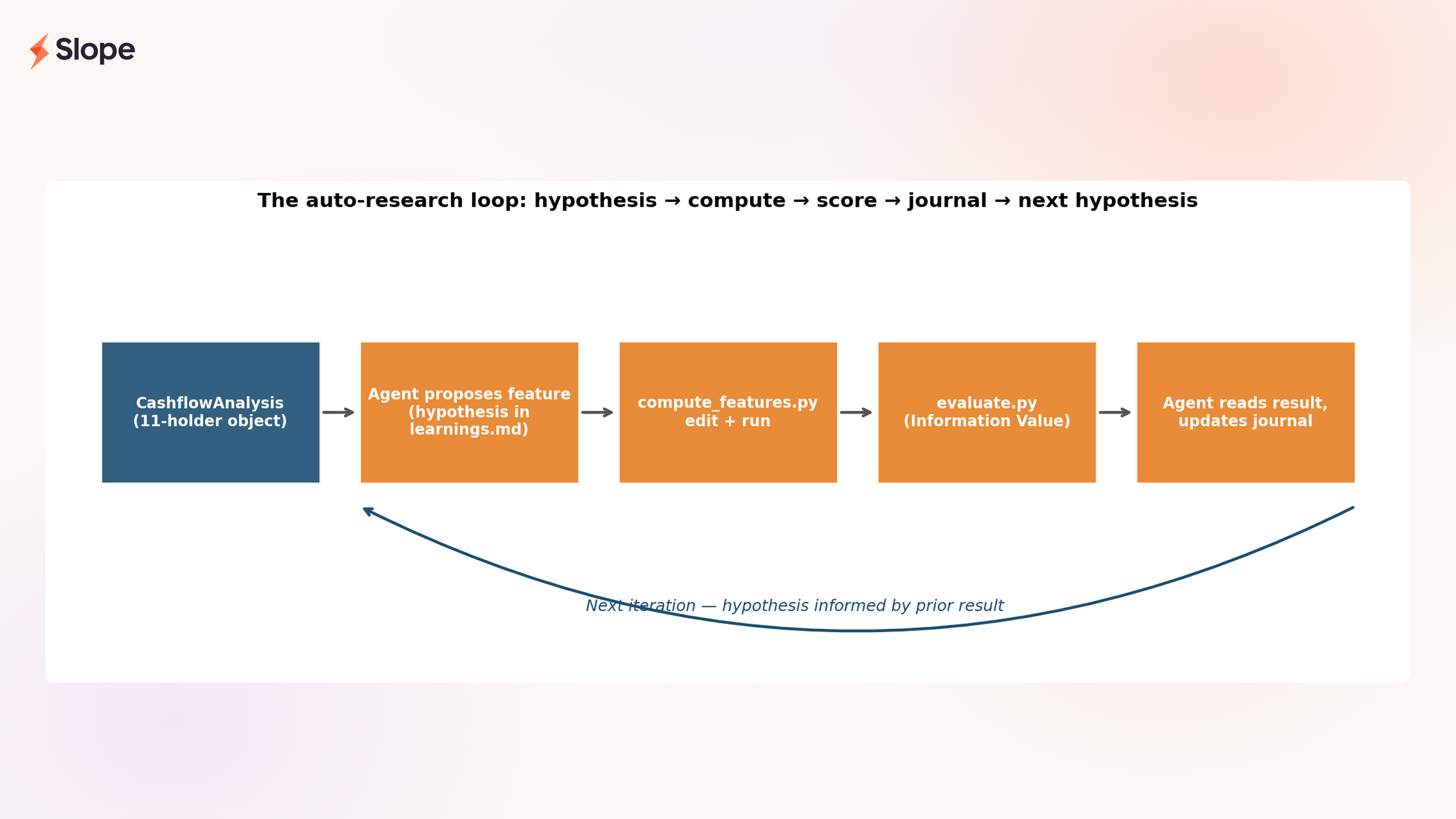
The inputs and outputs are deliberately narrow. The agent reads our CashflowAnalysis object, a structured, holder-based view of a customer's bank data that classifies every significant counterparty into one of eleven economic roles (revenue, COGS, payroll, debt, and so on). It writes features that are pure functions of that object. It scores them with Information Value against our own labeled customer data. It journals its reasoning. Then it goes again.

Three files, one cycle

The whole loop is implemented in three files, each with a single responsibility to keep the agent's job unambiguous.

• compute_features.py — the only file the agent edits. It takes a CashflowAnalysis object and returns a dict of scalar features.
• evaluate.py — fixed. Computes the Information Value of each feature against our labeled customer data, plus head-to-head comparisons against any analog in our existing feature set.
• learnings.md — the agent's research journal. Every iteration begins with a hypothesis stated in economic terms, and ends with a result, surprises, and what to try next.

Here is a real excerpt, lightly formatted, from iteration 8:

Hypothesis: Composite interactions (quality divided by distress, quality divided by debt, healthy-source count) will push more features into strong territory. Drop confirmed weak features (gross_margin_3m, payroll_ratio, cp_classification_coverage).

Top features by IV: is_window_count (0.600), distress_adjusted_quality (0.417), rev_recurrence_quality_score (0.386), quality_to_debt_ratio (0.375)

Surprises: distress_adjusted_quality (0.4174 STRONG!) — rev_recurrence_quality_score / (1 + distress_combined). Penalizing quality for opacity is highly discriminative. Now 2nd best feature overall.

That's the shape of every iteration. A testable economic claim, a measurement, a surprise log, and a list of what to try next. The IV score tests the reasoning, and features without a story get dropped regardless of how they score.

Three iterations, showing the reasoning

Let me walk through three iterations to make it concrete.

Iteration 6 — breadth × quality is better than breadth or quality alone

Hypothesis: A business with five reliable revenue sources is structurally safer than one with a single reliable source or five sporadic ones. Neither count alone nor recurrence alone captures this, you want their product.

Feature: rev_recurrence_quality_score = rev_source_count × rev_weighted_recurrence

Result: IV 0.386 (strong). The composite beat both of its components, rev_source_count came in at 0.313 and weighted recurrence was lower. A business with five sources at 0.8 recurrence scores 4.0 on this; a business with one source at 0.8 scores 0.8. Concentration risk and source quality, both expressed in a single number the model can read.

Importantly, this is not an algebraic trick. It's the whiteboard answer to "what do I actually mean when I say a business has reliable revenue?" Breadth and quality, not either one.

Iteration 8 — distress and debt act as penalties on quality

Hypothesis: Two businesses might have identical revenue quality scores, but one is opaque (high agent_review_ratio, high suspicious_inflow_ratio) and the other is not. The opaque one should have its quality score discounted, because opacity is a risk multiplier in credit (we don't know what we don't know). The same logic applies to debt burden: quality counts for less when the business is already servicing heavy obligations.

Feature: distress_adjusted_quality = rev_recurrence_quality_score / (1 + distress_combined), paired with quality_to_debt_ratio = rev_recurrence_quality_score / (debt_service_ratio + 0.1)

Result: IV 0.417 and 0.375. Both immediately landed in the top four features. The median IV across all features in the research jumped more this iteration than any other, a structural improvement in the feature set.

The economics here are the interaction a credit officer would draw on a whiteboard. Quality doesn't exist in a vacuum; it exists relative to what could eat it. The loop identified the interaction; the hypothesis told it where to look.

Iteration 25 — plateau, and the feature that defines the round

By iteration 25, the research had converged. For five consecutive iterations no new strong feature had emerged in this domain, which was exactly the stopping signal we'd written into the loop. We called the round complete with 58 strong features (IV ≥ 0.30) and 121 features total.

The feature that sits at the top of the new set — ontime_stability_score, IV 0.467 — is the one I'd want to call out to anyone skeptical about whether auto-research can produce features a credit officer would trust. It measures how consistently a customer's recurring revenue sources arrive on time, weighted by their share of total revenue. In plain terms: when business is hard, do you still pay on schedule? That is exactly what an experienced underwriter would tell you is the sharpest behavioral discriminator in a cashflow stream. The loop didn't discover a clever mathematical combination nobody had heard of. It built an operational version of an intuition the industry already agrees on, and proved it was the most predictive new signal in the round.

What the round produced

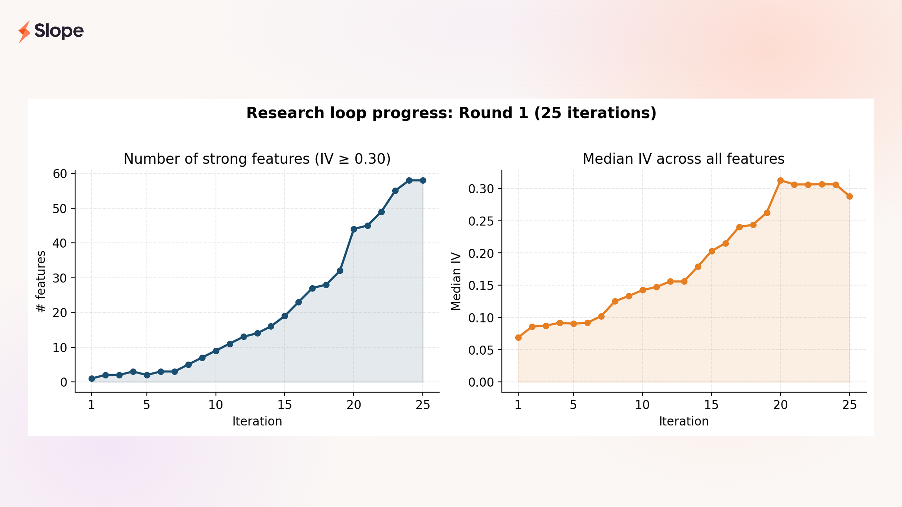
The left panel shows what the loop is actually for: growing the stock of strong features in the portfolio. Round 1 started with a single strong feature and ended with 58. The right panel, median IV across the whole feature set, is the quality counterpart. The average informativeness of the whole engineered feature set rose fourfold.

Looking at the composition of our final combined feature set:

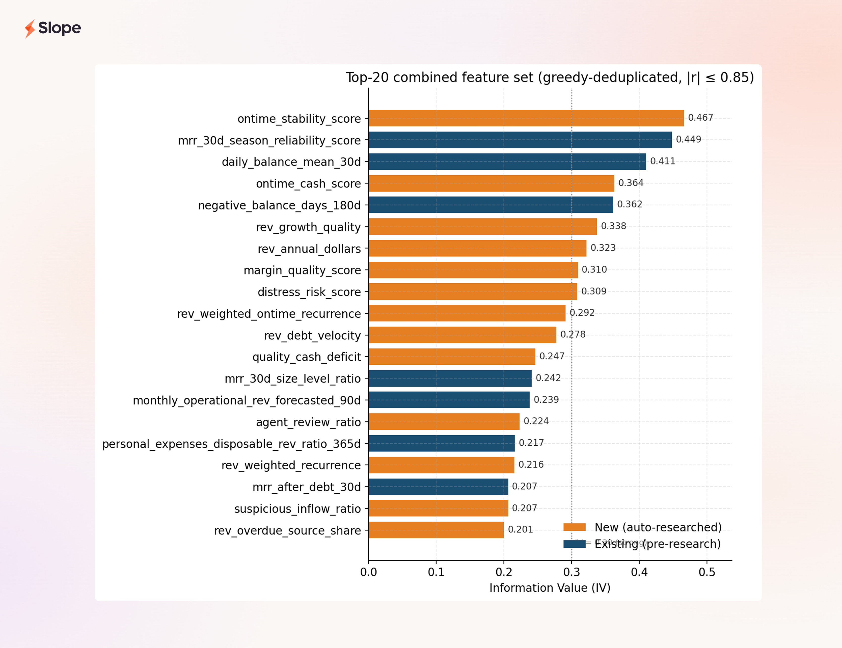
The top twenty features after greedy deduplication at |r| ≤ 0.85 (that is, twenty independent signals) contain twelve new auto-researched features and eight existing features. ontime_stability_score is now the single most predictive feature we have, new or old. And the mean Spearman correlation between the new features and our existing ones is 0.134, meaningfully orthogonal. These aren't re-expressions of balance or MRR. They're new axes.

The model lift:

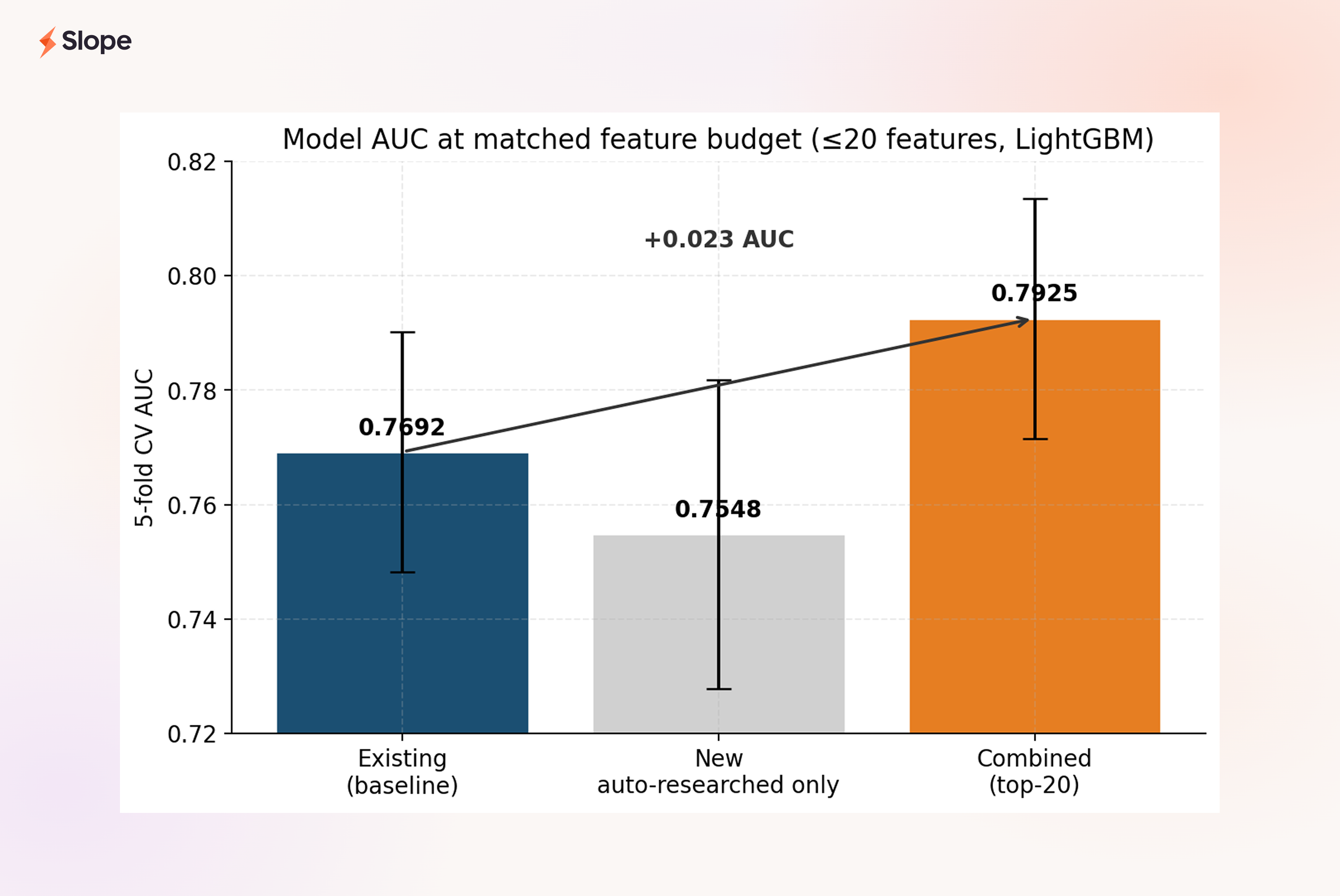
At the same budget of twenty features, the combined set beats the existing-only baseline by 0.023 AUC. In absolute terms this looks modest. At this range of the ROC curve, where we already sit at ~0.77, it is a substantial lift, and it comes from features that each have an economic rationale a credit officer can defend.

One thing worth noting: the new features alone (middle bar) slightly underperform the existing-only set. This is the right result. It tells us the new features are complementary, not a replacement. The balance and MRR features in the existing set carry signal the new quality scores don't fully replicate. The interesting story is the combined model, and that's where the lift lives.

Why this isn't brute-force feature engineering

The question a thoughtful reader will ask at this point is "isn't this just IV-chasing with extra steps?" It's the right question. Having the AI propose many candidates and keeping the ones that score well would, in fact, be data dredging at scale. Three design choices stop that from being what's happening here.

Hypothesis precedes measurement. Every iteration in learnings.md begins with an economic claim, a sentence you could read aloud to a credit committee. Features are proposed because of the claim, not selected after the scoring. If a feature scores strong IV but there's no clean hypothesis behind it, we drop it. The point of the loop is not to find correlations; it is to test ideas.

Composites require a mechanism. The distress-adjusted quality score isn't quality ⊕ distress for some arbitrary operator ⊕. It's quality / (1 + distress) because the economic mechanism is distress multiplies risk. Opacity doesn't add to revenue quality concerns; it divides it. The functional form has to match the mechanism, or we don't build it. This is the single most important discipline in the loop, and the one that most clearly separates principled feature engineering from throwing math at a wall.

Every feature passes the credit-officer test. Could a seasoned underwriter read the feature name, read the one-sentence definition, and say "yes, that should matter"? If not, we cut it, regardless of what the IV says. This sounds soft but it has teeth. It's why is_window_count, despite being the single highest-IV feature in the whole set, was not included among the "interesting" features we'd write a story about: it's a demographic control, not a behavioral signal, and a credit officer would shrug at it. IV-alone doesn't get to promote a feature. Defensibility does.

Together, these three guardrails turn "the agent can test many hypotheses quickly" into "the agent runs a disciplined research process quickly." The speed is AI's contribution. The discipline is the design of the loop.

What changes, and what's next

The biggest change from Round 1 is structural. Feature research is no longer a bottleneck. Round 2 is already running on balance-dynamics signals, a whole dimension the current feature set barely touches, and it's running at a cadence where each night's iterations feed the next morning's thinking. Features that used to take a week to evaluate now take minutes.

But the deeper change is cultural. The job of a DS on this project has shifted. Less time writing one feature, more time shaping the research direction, setting guardrails, and deciding which of the loop's proposals merit promotion. Less of the work that was hard because it was tedious; more of the work that's hard because it requires judgment.

The other thing worth naming explicitly: every feature in this post is a function of the CashflowAnalysis object, and that object is only as good as the labels underneath it. None of this works if the "recurring revenue" holder is polluted with loan disbursements, or if the "COGS" bucket doesn't see credit-card-funded inventory purchases for what they are. That's the subject of the next post in this series: the context-reasoning layer we've added on top of Slope Transformer that keeps these holder totals trustworthy. Cleaner labels, sharper features, better decisions.

Taken together, the two posts are my answer to a question I've been chewing on for a while: what does the 2026-era DS toolkit actually look like for small-business cashflow underwriting? It looks like an auto-research loop that mines our structured cashflow view for features the traditional model can use, and a context-reasoning layer that cleans up what text labels alone miss. Neither piece is revolutionary on its own. What's different is that a small focused team can now do both kinds of work at a pace that simply wasn't possible two years ago. I feel lucky to be pointing all of it at a problem that matters, and I'm looking forward to writing up what comes next.

— Jason Huang, CFA, Data Science at Slope